(c) Philip Gibbs
http://www.public.iastate.edu/~physics/sci.physics/faq/light-mill.html
LightMill image and animation by Torsten Hiddessen

Particles E= 1 2 mv2 p=mv=2E/v Photons E=hn p=E/c

History of (radiation driven) stellar winds

Wolf & Rayet	1867	class of stars with very broad spectral lines
Milne	1926	new plasma instability in the solar chromosphere
Beals Chandrasekhar	1929 1934	broad emission lines from W-R stars form in continuous outflow
Parker	1958 1960	hydrodynamics (!) of transonic (!) solar wind
[space borne UV spectrographs]	1967	P Cygni lines from O stars
Lucy & Solomon Castor, Abbott & Klein	1970 1975	stationary wind theory via radiative line driving
Abbott, Hamann, Hillier, Hummer, Kudritzki, Lucy, Owocki, Pauldrach, Puls, Rybicki	1980 - now	complex radiative transfer and non-LTE wind models including >100.000 lines, atmospheric blocking, multiline processes,...
Begelman, Norman, Shlosman, Turnshek, Weymann	again 1980 - now	radiation driven winds from accretion disks in quasars, cataclysmic variables, & young stellar objects

Recent interests in line driven hydrodynamics

	Shocks from the line driven instability Owocki et al. 1988 ApJ
	Wind compressed disks Bjorkman & Cassinelli 1993 ApJ
	Corotating interaction regions Cranmer & Owocki 1996 ApJ
	High-mass X-ray binaries Blondin et al. 1990 ApJ
	Quasar winds Murray et al. 1995 ApJ
	Disk winds Feldmeier & Drew 2000 MNRAS
	Thin winds Krticka & Kubat 2000 A&A

The minimum formalism

For a planar, one-dimensional wind

at zero sound speed,

the continuity and Euler equations become

in Sobolev approximation,

assuming a CAK line distribution

(F the stellar flux, C force constant, 0 < alpha < 1):

Hydronumerics of the CAK solution

Fortran hydrodynamics code for
solar wind and
radiation driven wind after CAK

The non-linear appearence of dv/dz
makes line driving almost as rich
as the Lorentz force in MHD

Especially, a new wave type occurs:
Abbott waves

And a new type of instability:
de-shadowing instability

DE-SHADOWING INSTABILITY AND ABBOTT WAVES

(back to start)



(Please klick on the image)




Consider a short scale perturbation which accelerates a fluid parcel to larger speeds. The perturbation gets amplified, since the parcel sees more stellar light ("unshadowing") and experiences a larger line force, which accelerates it further. This is the line driven instability.




Consider a large scale perturbation of the wind velocity law. At the node where the velocity gradients steepens, the Sobolev line force increases. The gas is accelerated to larger speeds ("upwards"), hence the node shifts inwards. This corresponds to an inward phase propagation, or a (marginally stable) Abbott wave. The same occurs at a node where the velocity law becomes shallower.

Unshadowing instability of thermal band: short wavelength limit (Lucy & Solomon 1970 ApJ)

Stable waves from 1st order Sobolev: long wavelength limit (Abbott 1980 ApJ)

Bridging law from exact (!) line transfer (Owocki & Rybicki 1984 ApJ) Unstable waves from 2nd order Sobolev (Feldmeier 1998 A&A)

Four forces

Up to now, four formulations of the line driving force g_l were given, of increasing complexity:

Sobolev force (simple)	SOB	Abbott waves, wind runaway
Pure absorption (complex)	ABS	Wind instability
Smooth source function force (complex)	SSF	Wind instability
Ensemble integrated source function force (very complex)	EISF	Instability, phase change, and Sobolev theory!

In general, an angle integral has to be applied.
For simplicity, we consider here only the force arising from radially streaming photons

f: Doppler line profile function
u: wind velocity, in units of thermal speed
x: normalized frequency, in Doppler units from line center
r: wind density
C: a constant


Sobolev force (Castor, Abbott, Klein 1975):
purely algebraic, on 50 spatial mesh points

gl = Cr-2    æ è r-1 du/dr ö ø a   ,             0 < a < 1

Pure absorption (Owocki, Castor, Rybicki 1988):
double integral on 5000 spatial × 50 frequency mesh points

gl = Cr-2 ó õ ¥ -¥  dx    f æ è x-u(r) ö ø é ë ó õ r   dr¢r(r¢) f æ è x-u(r¢) ö ø ù û a

SSF (Owocki 1991):
double integral on 5000 spatial × 50 frequency mesh points

gl = Cr-2 ó õ ¥ -¥  dx   f æ è x-u(r) ö ø æ ç è 1-S(r) t+a(x,r) + S(r) t-a(x,r) ö ÷ ø t+(x,r) = ó õ r   dr¢  r(r¢)  f æ è x-u(r¢) ö ø t-(x,r) = t max(r)  -  t+(x,r)

EISF (Owocki and Puls 1996):
four-fold integral on (5000 spatial × 50 frequency)² mesh points

Wind structure from numerical hydrodynamics

Owocki, Castor, Rybicki 1988 ApJ

ABS








Feldmeier 1994 Ap&SS

SSF

Generic wind model

The radial evolution of the wind

• from small radii, where perturbations are injected
• to large radii of fully developed structure
• to very large radii, where the structure decays

takes the form

Broad rarefactions regions of optically thin gas being accelerated to large speeds

Highly overdense shells (1-D simulat.) enclosed on inner side by starward facing reverse shocks which decelerate fast, rarefied gas

This structure is stable, since the rarefaction fins are optically thin and the gas in the shells decelerates whereas the unshadowing instability requires optically thick AND accelerating gas

GREENS FUNCTION

(back to start)


Owocki and Rybicki 1986:

Instead of dispersion analysis using sine waves

study wind response to localized perturbation:

Green's function.

	ABS Propagation of a smooth Gaussian pulse as an Abbott wave
	Reconstruction & propagation of the full Gaussian from a truncated one
	Reconstruction occurs only upstream of the localized perturbation = discontinuity. This truncated Gaussian vanishes upstream, hence nothing propagates

Information propagation?


BUT The O-R analysis is for pure absorption line driving.

In this case, it is trivial that no radiative wave propagates upstream. Hence, that no Abbott waves occur but only pure sound.

Nobody knows so far what happens for scattering lines beyond the Sobolev approximation...

X-RAYS AND CLOUD COLLISIONS

(back to start)


Corona model ruled out:

• no K-shell absorption observed
  (Cassinelli & Swank 1983)
  
  
• no green Fe XIV line observed
  (Baade & Lucy 1987)

Favored scenario:

X-ray source embedded in the wind

Random shock fronts

(Lucy 1980 ApJ; Cassinelli & Swank 1983 ApJ; Hillier et al. A&A 1994)

First problem with time-dependent wind models

Strong oscillatory thermal instability

(Langer et al. 1981 ApJ; Chevalier & Imamura 1982 ApJ)

leads to collapse of cooling zone on Eulerian mesh







Way out: modify cooling function artificially to have stable slope at low temperatures, irrelevant for X-ray emission

(Feldmeier 1994 Diss, 1995 A&A)

Second problem with time-dependent wind models

	density too small. Not enough X-rays (Hillier et al. 1994 A&A)
	solution: we propose (SSF) fast & dense cloudlets collide with shells (Feldmeier et al. 1997 A&A)

Wind model for zeta Ori, including energy transfer

Density, velocity and temperature snapshot at 3.5 days after model start.	Synthesised X-ray spectrum from this snapshot, compared to ROSAT data	The unique wind site responsible for this X-ray emission

(Please klick on the thumbnails for full-size images)

Evolution of wind structure in time

SSF

• Note numerous cloudlets in density plot
  
  
• ALL X-ray emission stems ONLY from cloudlet-shell collisions
  
  
• The snapshots above are at 3.5 days.
  Note the cloudlet collision between 6 and 7
  stellar radii in the wind evolution

(This movie file is too big for
net transport: available only on home machine)

X-ray lines with CHANDRA and XMM

The CHANDRA satellite



The LETG grating is a freestanding gold grating made of fine wires or bars with a regular spacing, or period , of 1 micrometer. The fine gold wires are held by two different support structures, a linear grid with 0.025 mm and a coarse triangular mesh with 2 mm spacing. The gratings are mounted onto a toroidal ring structure matched to the Chandra mirrors. The LETG gratings are designed to cover an energy range of 0.08 to 2 keV. However, their diffraction can also be seen in visible light, which is beautifully shown in the picture above right.





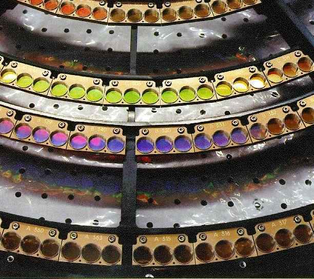
The CCD chip array with X-ray spectrum







XMM mirror, 3/4 (left picture) and fully (right picture) assembled



Application of X-ray CCDs in medicine:

X-RAY LINES

	CHANDRA: zeta Ori Waldron & Cassinelli 2001 ApJ counts vs. Angstrom
	CHANDRA: Theta 1 Ori C Schulz et al. 2001 ApJ
	CHANDRA: zeta Pup Cassinelli et al. 2001 ApJ counts vs. Angstrom
	XMM: zeta Pup Kahn et al. 2001 A&A

From Cassinelli et al. 2001, ApJ, 554, L55:

``...causes hot, X-ray emitting gas to be distributed throughout the dense stellar wind of zeta Pup and other OB stars. Wind-shock models developed by Lucy & White (1980), Feldmeier et al. (1997a), and others consistently failed to predict the high levels of X-ray emission observed in the brightest O stars like zeta Pup, leading to the suggestion that perturbations somehow form and propagate up from the photosphere into the wind and drive stronger shocks (Feldmeier 1995; Feldmeier, Puls, & Pauldrach 1997b). Broadband X-ray observations of zeta Pup (Corcoran et al. 1993; Hillier et al. 1993) indicate that some wind attenuation is affecting the soft X-ray flux. However, with the...''

	Wind shell frag- mentation
	global picture (Feldmeier et al. 2003, A&A)

X-RAY EMISSION LINE PROFILES








top: opt thin wind - bottom: opt thick wind

full: fragmented - dotted: homogeneous



(from Feldmeier et al. 2003, A&A)


Front view of radially randomized fragments:







Sky projection of radially randomized fragments. The front hemisphere of a unit sphere is cut into 16 384 roughly equal spherical triangles, which are subsequently randomly redistributed between r = 0.8 and 1.0 while their angular position is kept.

(from Oskinova et al. 2004, A&A)











Hidden opacity (Oskinova et al. 2007, A&:A):









Reason: opacity is hidden in highly compressed clumps






Note: density-squared diagnostics overestimates mass-loss

ION DECOUPLING AND RUNAWAY

(back to start)

History

Chandrasekhar	1943	Dynamical friction: momentum exchange due to gravitational force
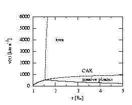
Castor, Abbott, & Klein	1976	Coulomb interactions between rad-driven ions and protons cease in thin winds
Springmann & Pauldrach	1992	Ion runaway after decoupling (see plasma literature of 1950ies)
Krticka & Kubat	2000	Ions and protons switch together (one fluid!) to slow solution branch
Owocki & Puls	2002	Technically, this is a shallow, subabbottic solution. Stability?
Votruba, Feldmeier, & Kubat	2007	Time-dependent hydrodynamic simulations of 2-component plasma

Work done: approximate Chandrasekhar function

in order that analytic = semi-implicit solution is possible

friction is 2nd derivative; leads to prohibitively short Courant time step

ABBOTT WAVES AND RUNAWAY

(back to start)


From now on till end: simple SOBolev line force

Question

Why does wind adopt unique, critical solution out of an infinite number of shallow and steep solutions?

Answer: Castor et al. 1975 ApJ

• Shallow solutions do not reach infinity
  because of backpressure
  
  
  
• Steep solutions do not reach photosphere
  because they start supersonically
  
  
  
• Hence, the true wind starts shallow,
  and switches at a critical point
  smoothly to a steep solution

Further evidence: Abbott 1980 ApJ

The CAK critical point is

to line-driven (Abbott) waves

what the sonic point is to sound waves:

an information barrier.

Concern

• Simulations out to 10 stellar radii
  converge to the CAK solution.
  But shallow solutions should be fine
  out to 300 stellar radii.
  
  (Plase klick on the image to see a movie)
  
  Artificial convergence to the CAK solution
  when pure outflow boundary conditions are used,
  and Abbott waves are NOT included in the Courant time step.
  
  
  SOB
  
  
  
• For disk winds, the critical solution
  fails to reach infinity, as do shallow
  solutions (Feldmeier & Shlosman 1999 ApJ).

Proposed runaway

towards critical solution (Feldmeier & Shlosman 2000)

Strange dispersion of Abbott waves: Positive velocity slopes propagate inwards Negative slopes propagate outwards Resulting in systematic acceleration of the wind: runaway

Runaway due to strange Abbott wave dispersion: schematic


SOB



Runaway in a numerical simulation. A periodic, sawtooth-like perturbation is maintained at x=2







The critical wind, however, is stable:



A sawtooth perturbation at x=2 with amplitude 5% creates inward propagating Abbott waves, but causes no runaway.



The same perturbation but with amplitude 15% causes runaway. (The horizontal velocity law beyond x=2 is an artifact of the applied boundary conditions.)


SOB

Runaway terminates when critical point forms

and shuts off Abbott wave propagation towards the photosphere.

If perturbations occur below the critical point

runaway proceeds to overloaded solutions

with supercritical mass loss rate

until a generalized critical point forms.

Overloaded solutions can become stationary.

A perturbation at x=0.8, below the critical point at x=1. The runaway proceeds to an overloaded solution. In the broad region with negative velocity gradient, gravity overcomes the line force. The period of the perturbation is here ten times shorter than above.


SOB

SOURCE FUNCTION ITERATION

(back to start)

Rybicki & Hummer (1978) considered v=1/r with resonance surface (multiple radiative coupling!)



For a linear-hyperbolic-linear velocity law (e.g. due to overloading) the shape of the resonance surface is



...and in the neighborhood of the outer kink.

Basic equations

	Pure absorption force Owocki, Castor, & Rybicki 1988 ApJ
	Smooth Source Function: Sobolev Owocki 1991
	Iterated source function Rybicki & Hummer 1978 ApJ
	Iterated SF for 3-point coupling Feldmeier & Nikutta 2006 A&A
	Alternative method Baron & Hauschildt 2004

The wind structure after S-iteration (thick line) vs CAK wind (thin line) is

ABBOTT SHOCKS

(back to start)


Ongoing work with Dennis Raetzel



Cranmer & Owocki 1996 ApJ

DISK WINDS

(back to start)


still: SOB


Winds from accretion disks in

• Protostars
• Cataclysmic variables
• Quasars

Simplifying assumption so far: protostellar winds are magnetically driven...

... winds from cataclysmic variables are line driven.

Here: combination of magnetic and radiative driving

Two basic differences between star and disk wind launching

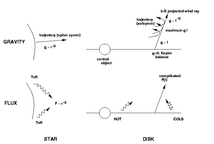
Gravity and radiation flux have independent maxima as function of height: up to 3 critical points. (For stars: 1)

Short history of papers on line driven disk winds

Shlosman 1985. Quasar winds with local launching due to disk radiative flux. Bright central region is shielded by absorption in disk atmosphere.

Shlosman & Vitello 1988. There is no critical point for vertical launching ... (and many more approximations) -> Ionization gradients central?

de Kool & Begelmann 1994. Similarity solution for magnetic wind with scaled-up continuum radiation driving (no true line driving).

Feldmeier & Shlosman 1999. Analytical solution along straight wind cones. 2-D eigenvalue problem: mass loss rate and wind tilt angle.

Proga, Stone & Drew 1998. First time-dependent wind models using Zeus 2-D code.

(another) disk wind movie

Results for line driven disk winds at B=0

1. mass loss rates in good agreement with CAK theory
   
   
2. however: much smaller than single scattering limit : thin winds
   
   
3. inherent wind variability: streamers. Origin unclear

Recent MHD + rad hydro simulations

Central questions:

• can magnetic field increase mass loss?: B=0 winds are presently far too thin
  
  
• can radiative launching overcome problems with pure magneto-thermal launching? (Ogilvie & Livio 1998)

Classical scenario for MHD winds

magnetic pressure >> gas pressure ("corona")

-->

corotating, rigid poloidal magnetic field lines

-->

for tilts > 30 deg, gas flows away freely from the disk:

(gas) beads on a (magnetic) wire

Surprisingly

we find that Zeus 2-D favors another flow scenario first suggested theoretically by Contopoulos 1995.

Here, only a toroidal magnetic fields occurs.

Wind is launched via Lorentz force due to vertical gradients of the toroidal field. By contrast, Blandford & Payne wind is launched via centrifugal force due to stiff poloidal field lines.

The Lorentz force j x B ~ (rot B) x B points upwards.

A dynamical mixture of Blandford-Payne and Contopoulos winds?

Our models show an interplay between poloidal and toroidal fields:

only for sufficiently strong poloidal fields, a Kelvin-Helmholtz vortex sheet forms

at the edge of the star with the disk, and extending outwards at a polar angle of 45 deg.

The K-H eddies carry the toroidal field above the CAK critical point

which corresponds to the bottleneck of the flow.

The Lorentz force from the toroidal field can then assist in carrying enhanced mass loss.

By contrast, models with pure toroidal fiels (pure Contopoulos model) show smaller, CAK mass loss rates.

Kelvin- Helmholtz wave in poloidal magnetic field unit arrow (top right) = 0.5 Gauss please click on the image to see the movie