Details of the SMC-OB-Vd3 models

The main parameters for OB-star atmospheres are the stellar temperature T and the surface gravity g_grav. These two parameters span the plane of the model grid in steps of 1 kK in temperature and 0.2 dex in surface gravity.

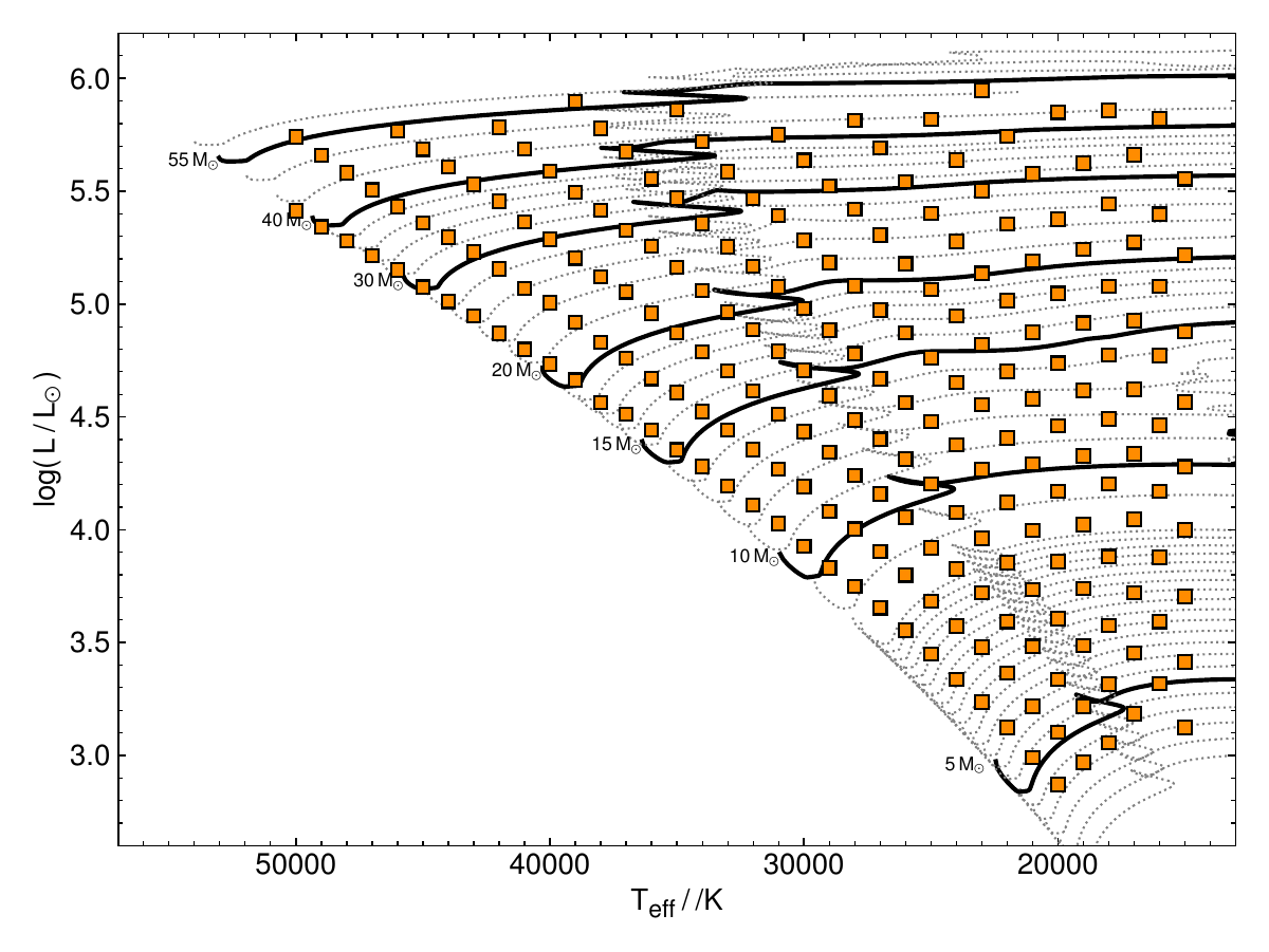
Furthermore, there are parameters of secondary importance (e.g. the luminosity of the star), which influence the appearance of the emergent spectra. In order to specify the stellar luminosity and mass at given T and log g_grav, we apply the non-rotating stellar evolution models (MESA Isochrones and Stellar Tracks; MIST) from Choi et al. 2016. Consequently, our model grid is restricted to parameters that are reached by these tracks for single-star evolution. In Figure 1 we display these tracks in the HRD, over-plotted by the final positions of the individual grid models.

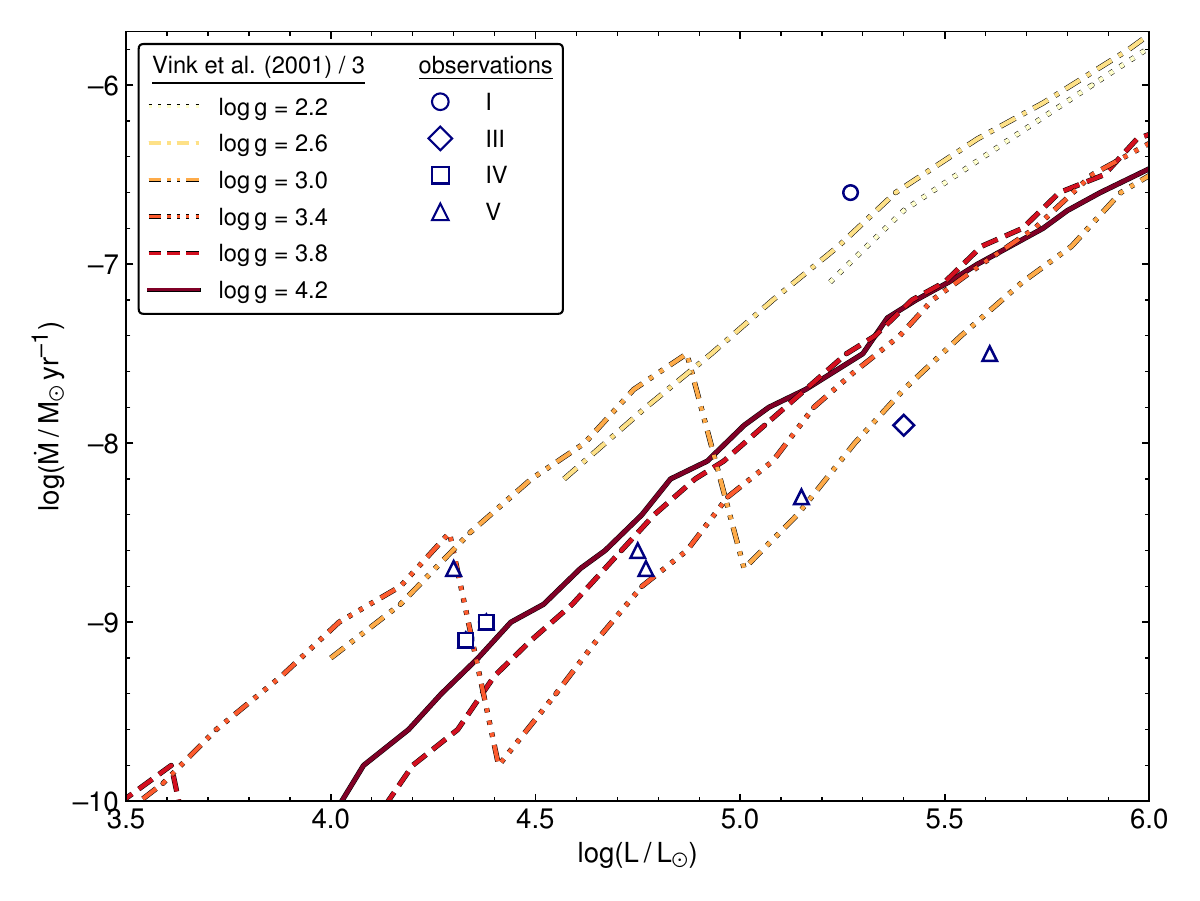
**Figure 1:** HRD showing the MIST evolutionary tracks at SMC metallicity (lines), over-plotted by the positions of the grid models (squares). We show all MIST tracks in the initial mass-range of M = 4-60 M. For clarity, we highlight the tracks with initial masses of 5 M, 10 M, 15 M, 20 M 30 M, 40 M and 55 M as black solid lines, while the remaining tracks are represented by gray dotted lines.

Further parameters with potential influence on the spectra are the mass-loss rates M and the terminal wind velocity v. For specifying the mass-loss rate we adopt the recipe by Vink et al. (2001) - their Eqs. 24 and 25 for the hot and cool side of the bi-stability jump. The terminal wind velocity v is adopted to be proportional to the escape velocity v_esc. As recommended by Vink et al. (2001), the proportionality factor is set to v = 2.6 v_esc and v = 1.3 v_esc for the hot and cool side of the bi-stability jump, respectively.

Recent empicial studies (e.g. Ramachandran et al. 2019, Rickard et al. 2022) have shown that OB-star winds in the SMC are in fact much weaker than the original recipe predicts. Therefore, we divide the predicted M by a factor 3, yielding a better agreement across the various luminosity classes (see Fig. 2).

**Figure 2:** Vink et al. (2001) mass-loss rates for different sets of surface gravities (lines), compared to empicial measurements of O-type stars ind the SMC (symbols) adopted from Ramachandran et al. 2019.

The model calculations account for inhomogeneities in the stellar wind (micro-clumping). Clumping is assumed to set in at the sonic point and to reach the full clumping factor of D = 10 at a radial distance of 10 R.

The abundances of C, N, O, Mg, Si, and Fe are obtained from Trundle et al. (2007). The abundances of the other trace elements are adopted as 1/7 Z, referring to the solar abundances from Asplund et al. (2009) (c.f. TMAP abundance list). The ionization stages that are taken into account are optimized according to the model's effective temperature, as documented in the tables below.

Summary of the employed model atoms:

T < 21.5 kK
Ion		No. of levels
H I	22
H II	1
He I	35
He II	26
He III	1
N I	10
N II	38
N III	56
N IV	6
N V	0
N VI	0
C I	15
C II	32
C III	40
C IV	25
C V	1
C VI	0
O I	13
O II	37
O III	33
O IV	2
O V	0
O VI	0
S II	32
S III	23
S IV	25
S V	1
S VI	0
S VII	0
Mg II	32
Mg III	43
Mg IV	0
Mg V	0
Si II	20
Si III	24
Si IV	23
Si V	1
Si VI	0
Si VII	0
P III	47
P IV	12
P V	3
P VI	0
G I	1
G II	3
G III	13
G IV	18
G V	1
G VI	0
G VII	0
G VIII	0
G IX	0

21.5 kK < T < 28.5kK
Ion		No. of levels
H I	22
H II	1
He I	35
He II	26
He III	1
N I	10
N II	38
N III	56
N IV	38
N V	2
N VI	0
C I	15
C II	32
C III	40
C IV	25
C V	1
C VI	0
O I	13
O II	37
O III	33
O IV	29
O V	2
O VI	0
S II	32
S III	23
S IV	25
S V	20
S VI	1
S VII	0
Mg II	32
Mg III	43
Mg IV	0
Mg V	0
Si II	20
Si III	24
Si IV	23
Si V	52
Si VI	0
Si VII	0
P III	47
P IV	12
P V	11
P VI	1
G I	0
G II	1
G III	13
G IV	18
G V	22
G VI	1
G VII	0
G VIII	0
G IX	0

28.5 kK < T < 33.5 kK
Ion		No. of levels
H I	22
H II	1
He I	35
He II	26
He III	1
N I	10
N II	38
N III	56
N IV	38
N V	2
N VI	0
C I	15
C II	32
C III	40
C IV	25
C V	1
C VI	0
O I	13
O II	37
O III	33
O IV	29
O V	2
O VI	0
S II	32
S III	23
S IV	25
S V	20
S VI	22
S VII	1
Mg II	32
Mg III	43
Mg IV	1
Mg V	0
Si II	20
Si III	24
Si IV	23
Si V	52
Si VI	1
Si VII	0
P III	47
P IV	12
P V	11
P VI	1
G I	0
G II	1
G III	13
G IV	18
G V	22
G VI	29
G VII	1
G VIII	0
G IX	0

33.5 kK < T < 38.5 kK
Ion		No. of levels
H I	22
H II	1
He I	35
He II	26
He III	1
N I	0
N II	38
N III	56
N IV	38
N V	20
N VI	1
C I	0
C II	32
C III	40
C IV	25
C V	29
C VI	0
O I	0
O II	37
O III	33
O IV	29
O V	54
O VI	2
S II	0
S III	23
S IV	25
S V	20
S VI	22
S VII	1
Mg II	32
Mg III	43
Mg IV	1
Mg V	0
Si II	20
Si III	24
Si IV	23
Si V	52
Si VI	1
Si VII	0
P III	0
P IV	12
P V	11
P VI	1
G I	0
G II	1
G III	13
G IV	18
G V	22
G VI	29
G VII	19
G VIII	1
G IX	0

38.5 kK < T
Ion		No. of levels
H I	22
H II	1
He I	35
He II	26
He III	1
N I	0
N II	0
N III	56
N IV	38
N V	20
N VI	14
C I	0
C II	0
C III	40
C IV	25
C V	29
C VI	1
O I	0
O II	37
O III	33
O IV	29
O V	54
O VI	35
S II	0
S III	0
S IV	25
S V	20
S VI	22
S VII	15
Mg II	32
Mg III	43
Mg IV	17
Mg V	1
Si II	0
Si III	24
Si IV	23
Si V	52
Si VI	10
Si VII	1
P III	0
P IV	12
P V	11
P VI	1
G I	0
G II	0
G III	1
G IV	18
G V	22
G VI	29
G VII	19
G VIII	14
G IX	1

Notes: Element "G" stands for the generic iron-group element, which combines the elements from Sc to Ni in solar relative mixture. In case of the "G" element, the number of levels given in the above table actually refers to superlevels.

Contour plots

For a couple of lines, contour plots of the equivalent width have been prepared. The contours are labeled with W_λ in Angstroem:

logQ	HI	ps	pdf	png
logQ	HeI	ps	pdf	png
logQ	HeII	ps	pdf	png
H	α	ps	pdf	png
H	β	ps	pdf	png
He I	5876	ps	pdf	png
He II	4686	ps	pdf	png
He II	5412	ps	pdf	png